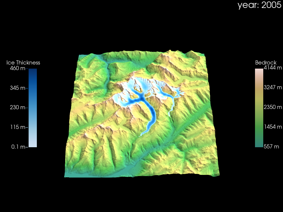
Getting started with Glacier:3D-Viz

This notebook gives you a quick overview of how to get started with Glacier:3D-Viz for creating 3D visualizations of dynamic glacier runs. Although it is designed to work seamlessly with native OGGM outputs, you can use any xarray.Dataset as long as it follows the data format guidelines described below.

Open input data for visualization

Glacier:3D-Viz is designed to work seamlessly with output generated by OGGM. However, if you want to create 3D glacier visualizations from purely measurements or other dynamic glacier models, you can do so. You only need to structure the NetCDF input data accordingly (below you can find an example using IGM output). Let’s have a look at an example (created and copied from this OGGM tutorial):

import xarray as xr

with xr.open_dataset("oggm_constant_climate_dummy_data.nc") as ds:
    ds_glacier = ds

You see the file has some coordinates and data variables, not all of them are needed for a minimum visualisation, but some of them are nice features for addons, shown at other points of the tutorials. The minimum data needed for the visualisation are the coordinates (x, y, time) and the data variables (bedrock, distributed_thickness). However, you can decide on the naming as they can be explicitly set during the creation of the 3D visualization object in the next step.

Create the 3D visualization object

Creating a 3D visualization object is quite easy. Just provide your data and define the names of the coordinates and data variables which should be used. The default variables are the ones used by OGGM (see example data above), but for demonstration, we set everything explicitly here:

from glacier3dviz.tools import Glacier3DViz

viz = Glacier3DViz(
    ds_glacier,  # dataset for visualization
    x='x',  # x-coordinate name, default is 'x'
    y='y',  # y-coordinate name, default is 'y'
    time='time',  # time coordinate name, default is 'time'
    topo_bedrock='bedrock',  # bedrock data variable, default is 'bedrock'
    ice_thickness='simulated_thickness',  # evolving ice thickness variable, default is 'simulated_thickness'
    time_var_display='calendar_year',  # time format displayed, opting for total years here
    camera_args={  # camera view settings, more details later
        'azimuth': -135, # rotate around the z-axis
        'elevation': 20,  # elevation angle above ground
    }
)

And thats all! Now lets see what we can do with the viz:

Interactive visualization in notebook

Opening an interactive visualization in the notebook and explore your data is straightforward. However, for this to work you must make sure that ipywidgets is correctly installed (https://ipywidgets.readthedocs.io/en/latest/user_install.html).

In the interactive visualization, you can use the slider to scroll through time, you can zoom and change the point of view, and finally, you can directly save it to an image.

The interactive viz.show() command currently does not display well in the Jupyter Book. You will get better results by executing the notebook locally. We are working on improving this!

viz.show()

Export animation

Or you can easily export it as an animation:

viz.export_animation(filename='dummy_animation.mp4',  # filename for the animation, should end with .mp4
                     framerate=20,  # framerate of the animation, affects duration and speed
                     quality=5,  # The range is 0 - 10. Higher quality leads to a larger file.
                    )

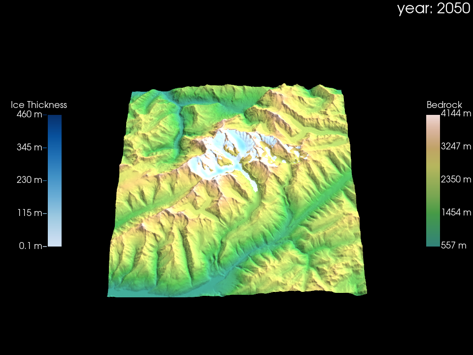
Plot a single year

Or extract some static plots of single years for static visualizations:

viz.plot_year(2050,  # year to visualize
              filepath='dummy_fig_2050.png',  # file path for saving the image; if not provided, displays in notebook only
              show_plot=True,  # whether to show the plot in the notebook when saved
             )

Visualizing IGM output

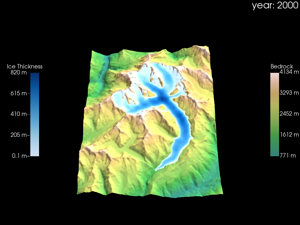
As an example of how Glacier:3D-Viz works with the output of a model other than OGGM, we provide an illustration using IGM output data. In principle, you just need to load the data as previously shown and adjust the variable names accordingly.

with xr.open_dataset('igm_dummy_data.nc') as ds:
    ds_igm_glacier = ds

viz_igm = Glacier3DViz(
    ds_igm_glacier,  # dataset for visualization
    x='x',  # x-coordinate name, default is 'x'
    y='y',  # y-coordinate name, default is 'y'
    time='time',  # time coordinate name, default is 'time'
    topo_bedrock='topg',  # bedrock data variable, default is 'bedrock'
    #use_texture=True,  # utilize background map (satellite imagery) for topography texture
    ice_thickness='thk',  # evolving ice thickness variable, default is 'simulated_thickness'
    time_var_display='time',  # time format displayed, opting for total years here
    camera_args={  # camera view settings, more details later
        'azimuth': -135, # rotate around the z-axis
        'elevation': 20,  # elevation angle above ground
    }
)

viz_igm.plot_year(2000)

Enriching the visualization

Creating simple visualizations with Glacier:3D-Viz is straightforward, but you may want to enhance these visuals by adapting the topography texture or adding annotations. For instance, incorporating satellite imagery for the topography or annotating geographic features can significantly enhance the visual impact. Below are two examples that demonstrate how to customize your visualization with various annotations and textures:

For more in-depth explanations on how to adapt and refine your visualizations as shown above, please refer to the following tutorials:

• General styling of 3D visualizations

• Annotating your 3D glacier visualizations

• Advanced Visualizations