General styling of 3D visualisations#
This notebook shows you how to change the general style of your plotting, including the size of the plot, colors, and the point of view. As the 3D tool is built around the fantastic PyVista package, many things shown here can be further adapted following the links to the PyVista documentation provided throughout this notebook.
For all options we change here, we also defined a set of default values. You can have a look at these default values by calling viz.example_arg_default to get a first overview of available options. For a more comprehensive overview use the link list provided below.
A general remark: all options presented here can be changed on the fly by providing the kwargs when calling, for example, .plot_year(), or you can provide them directly during the creation of the 3D object. Everything that is not provided falls back to the default values. This approach was intended to make it easy to play around while searching for your best setting, and once you found it, you can define it during creation of the 3D-object to make the following code for creating animations or plots easier.
PyVista documentation overview#
Throughout this notebook, we are referring to the PyVista documentation for getting an overview of which options are available for customization. Here, we provide a link collection to the PyVista documentation for recurring Glacier:3D-Viz users:
plotter_args: PyVista plotter documentationadd_mesh_ice_thick_args: PyVista add mesh documentationadd_mesh_topo_args: PyVista add mesh documentationvar_display_lookuptable_args: PyVista LookupTable documentationcamera_args: PyVista camera documentationlight_args: PyVista light documentationbackground_args: PyVista plotter set background documentationtext_time_args: PyVista plotter add text documentation
More information about these options is provided throughout this notebook.
Open data and create 3D object#
import xarray as xr
from glacier3dviz.tools import Glacier3DViz
ds_glacier = xr.open_dataset("oggm_constant_climate_dummy_data.nc")
viz = Glacier3DViz(
ds_glacier, # the dataset for visualisation
camera_args={ # arguments for the point of view
'azimuth': -135, # rotate the map around the z-axis
'elevation': 20, # set the elevation above ground of the point of view
}
)
Plotter arguments (e.g. window_size)#
The general visualization is made using a plotter, which can be customized using different arguments. For example, we can define the window_size of the final plot. For more options, check out the documentation of pyvista.plotter.
# have a look at the default settings
viz.plotter_args_default
{'window_size': [960, 720], 'border': False, 'lighting': 'three lights'}
# define a new wineow_size for the resulting plot
plotter_args_new = {'window_size': [650, 400]}
viz.plot_year(2050,
plotter_args=plotter_args_new)
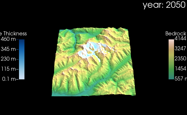
By changing the window size you probably also need to adapt the position of the colobars. How to do this is explained below.
Ice Thickness color & colorbar#
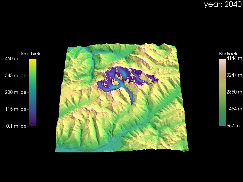
Here we show how to change the colors and style of the ice thickness and how to adapt the corresponding colorbar. We added ‘nice’ numbers to the colorbar (minimum value is 0.1 m, other labels are intagers ending with 0 or 5). For doing this we are using a PyVista LookupTable in combination of adding PyVista a mesh. Therefor we have list of arguments to change:
for the mesh it is called
add_mesh_ice_thick_argsfor the LookupTable it is called
var_display_lookuptable_args
# have a look at the default values
viz.add_mesh_ice_thick_args_default
{'scalar_bar_args': {'title': 'Ice Thickness ',
'n_labels': 0,
'color': 'white',
'vertical': True,
'position_x': 0.1,
'position_y': 0.3,
'height': 0.4},
'show_scalar_bar': True}
viz.var_display_lookuptable_args_default
{'cmap': <matplotlib.colors.ListedColormap at 0x7df232ff68d0>,
'n_labels': 5,
'scalar_range': [0.1, np.float64(460.0)],
'annotations': {np.float64(0.1): '0.1 m',
np.float64(115.07499999999999): '115 m',
np.float64(230.04999999999998): '230 m',
np.float64(345.025): '345 m',
np.float64(460.0): '460 m'}}
add_mesh_ice_thick_args_new = {
'scalar_bar_args': { # some arguments for the colorbar
'position_x': 0.12, # set x_position of colorbar
'title': 'Ice Thick ', # change the title, the whitespace is used to center the title
}
}
# create new annotations by adding Ice at the end
new_annotations = {key: value + ' Ice'
for key, value in viz.var_display_lookuptable_args_default['annotations'].items()
}
var_display_lookuptable_args_new = {
'cmap': 'viridis', # change the used colormap
'annotations': new_annotations, # add our new annotations
}
viz.plot_year(2040,
add_mesh_ice_thick_args=add_mesh_ice_thick_args_new,
var_display_lookuptable_args=var_display_lookuptable_args_new,
)
Color surface with custom variable#
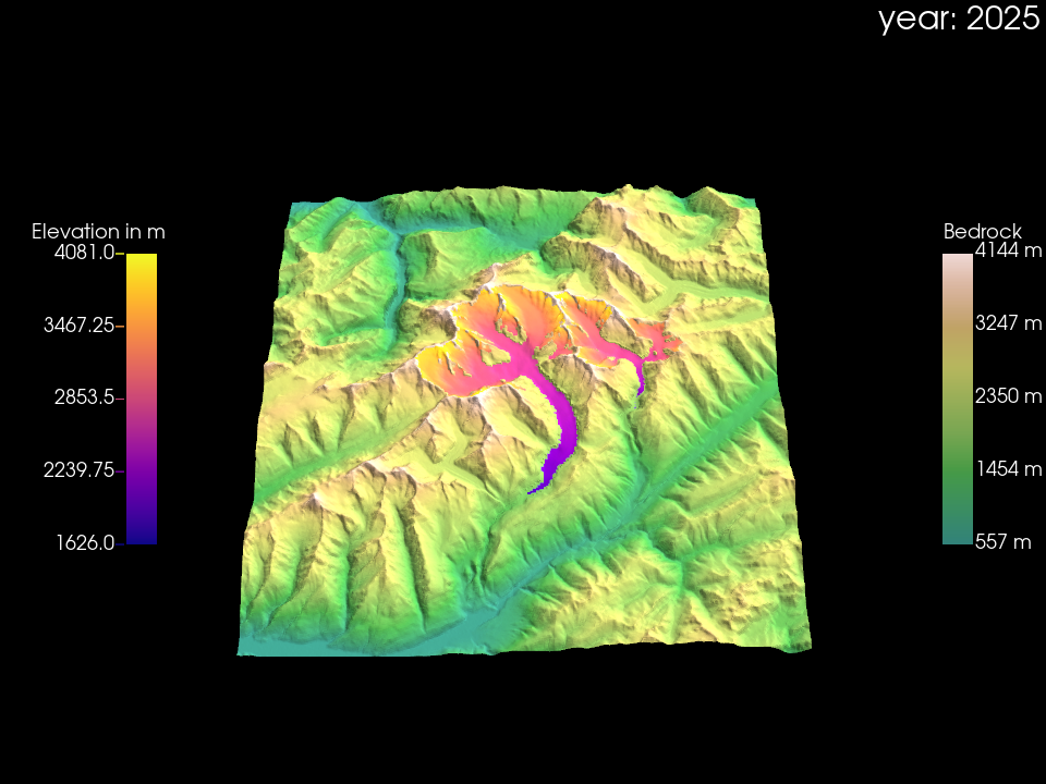
If you want to color the glacier surface using a custom variable, make sure the variable is included in the provided dataset and define it using var_display. You can also customize the colorbar as needed.
# change the title of the colorbar
add_mesh_ice_thick_args = viz.add_mesh_ice_thick_args_use
# adding 25 spaces for centering the title
add_mesh_ice_thick_args['scalar_bar_args']['title'] = 'Elevation in m' + ' ' * 25
viz.plot_year(2025,
var_display='topo',
add_mesh_ice_thick_args=add_mesh_ice_thick_args,
# use a different colormap
var_display_lookuptable_args={'cmap': 'plasma'},
)
Bed topography color and colorbar#
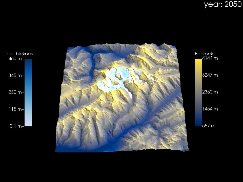
If you like to adapt the styling of the bed topography, here you can find an example how this can be done. However, you can also try out using satellite data for the coloring of the topography, explained in the next section. And as always have a look at the PyVista documentation for more options.
# have a look at the defaults
viz.add_mesh_topo_args_default
{'cmap': <matplotlib.colors.ListedColormap at 0x7df231a573b0>,
'scalar_bar_args': {'title': 'Bedrock',
'vertical': True,
'fmt': '%.0f m',
'color': 'white',
'position_x': 0.9,
'position_y': 0.3,
'height': 0.4},
'show_scalar_bar': True,
'texture': None}
add_mesh_topo_args_new = {
'cmap': 'cividis',
'scalar_bar_args': {
'position_x': 0.8,
}
}
viz.plot_year(2050,
add_mesh_topo_args=add_mesh_topo_args_new)
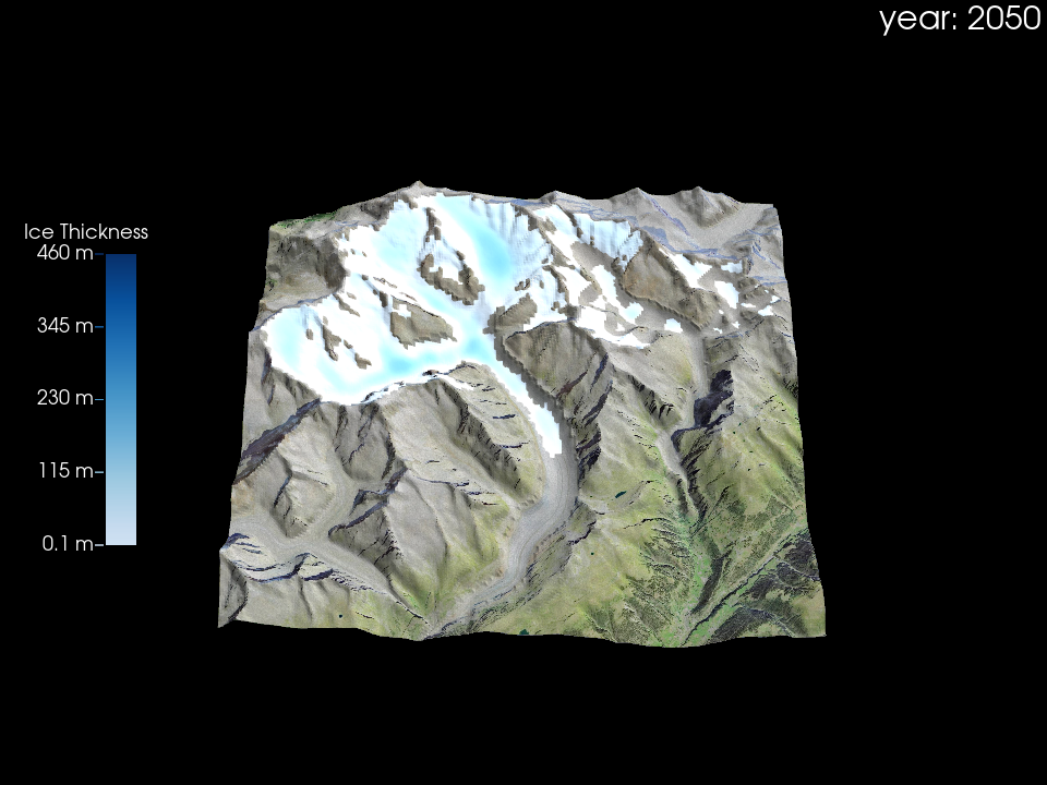
Bed topography texture from satellites#
A nice addition of Glacier:3D-Viz is that you can use bed topography from satellite data. However, currently this is only possible for a relative ‘small’ region, but we are working on a fix for this. Note, that for this we need to download some data and this might take some time. Once you have downloaded the data for your glacier and are adapting the styling further you can rely on the cached satellite data.
viz_satellite = Glacier3DViz(
ds_glacier.isel( # the dataset for visualisation, here we select a smaller extent
x=slice(120, 355),
y=slice(120, 340)),
use_texture=True, # decide to use background map (satellite imagery) for texture on the topography
camera_args={ # arguments for the point of view
'azimuth': -135, # rotate the map aroung the z-axis
'elevation': 20, # set the elevation above ground of the point of view
}
)
viz_satellite.plot_year(2050)
Change point of view#
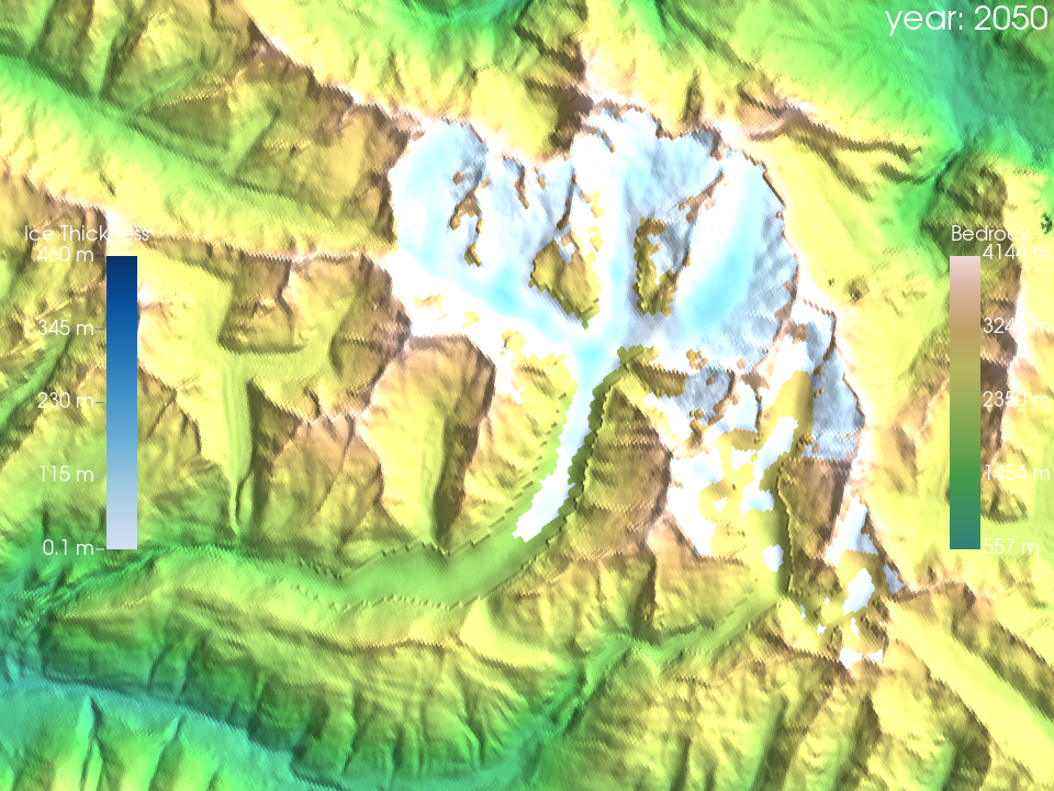
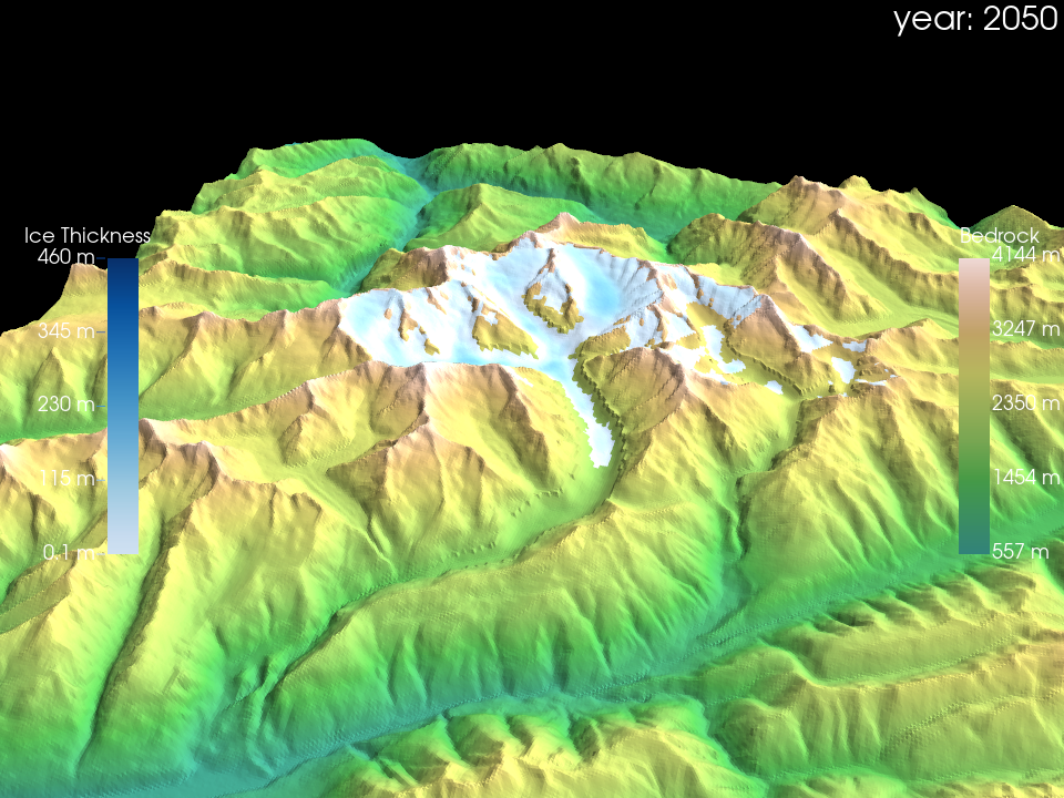
We already changed the camera position in the default initialisation of viz above. However, here once again explicitly showing some options, for more options checkout the PyVista documentation. You also can use the interactive viz.show() for searching for a position and read this out, as shown below.
# have a look at the defaults, we set during initialisation of viz
viz.camera_args_default
{'azimuth': -135, 'elevation': 20, 'zoom': 1.0, 'normalized_position': True}
camera_args_new = {
'azimuth': -80,
'elevation': 50,
'zoom': 2.5,
}
viz.plot_year(2050,
camera_args=camera_args_new)
viz.show() command currently does not display well in the Jupyter Book. You will get better results by executing the notebook locally. We are working on improving this!
viz.show()
# adapt the point of view you want to define above and call this cell afterwards to get the coordinates
viz.get_camera_position()
[0.0, -3.0259101390838623, 48.929161071777344]
# And use this position for your next plot, here an example
camera_args_new = {
'position': [0.7, -2, 16],
}
viz.plot_year(2050,
camera_args=camera_args_new)
Lighting#
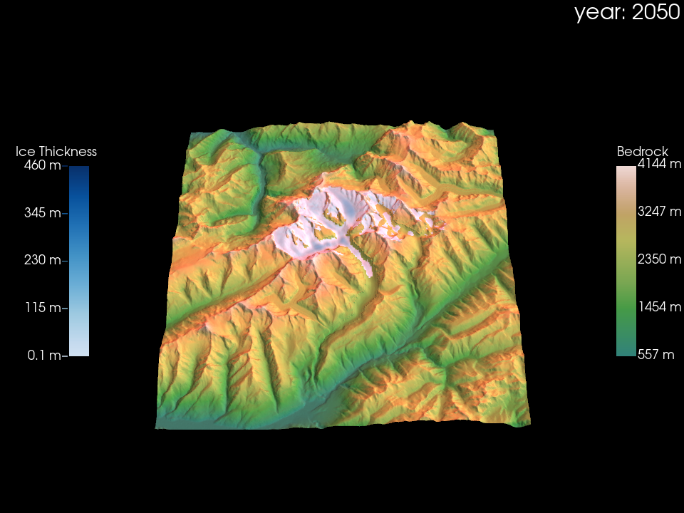
The lighting of the plot can be important depending on your point of view and on the features you want to highlight in your visualisaitons. A comprehensive list of posibilities can be found in the lightning documentation of PyVista.
# have a look at the defaults
viz.light_args_default
{'position': (0, 1, 1), 'light_type': 'scene light', 'intensity': 0.6}
light_args_new = {
'color': 'red'
}
viz.plot_year(2050,
light_args=light_args_new,
)
Background color#
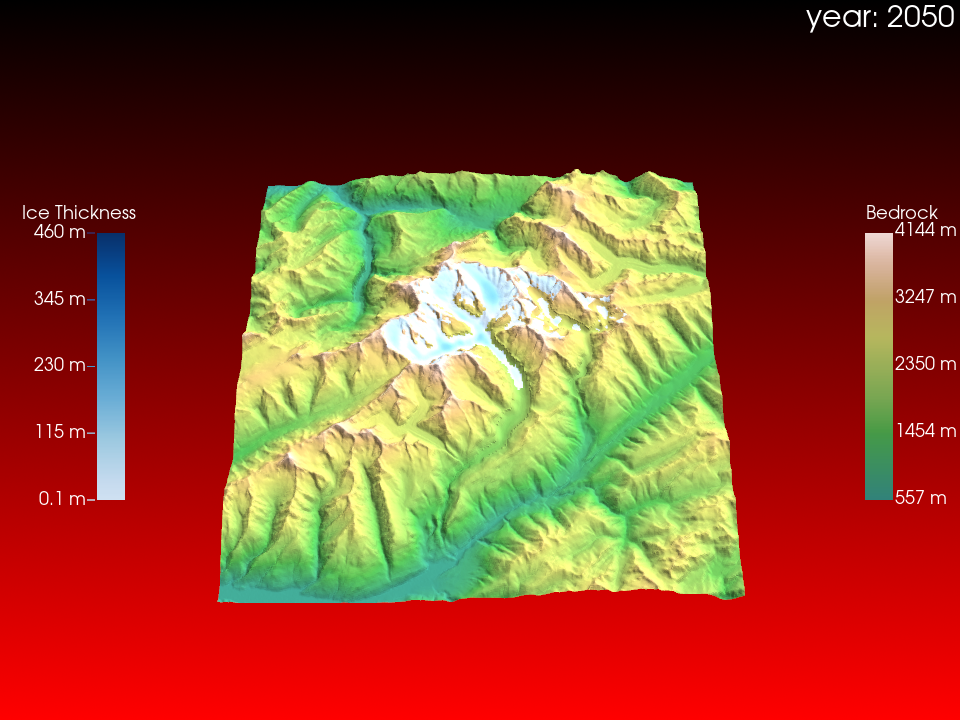
You might want to change the look of the background (default is black). Instead of one color you also could gradual shift from red to black, from bottom to top. You can set it as you wish, following the available options of the set_background documentation of pyvista.
# have a look at the defaults
viz.background_args_default
{'color': 'black'}
background_args_new = {
'color': 'red',
'top': 'black'
}
viz.plot_year(2050,
background_args=background_args_new)
Define extend of shown data#
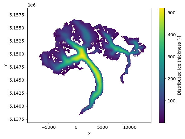
You can decide to show only part of your total dataset. For this you either can make a selection before providing the dataset to Glacier:3D-Viz:
ds_glacier_zoomed = ds_glacier.isel(x=slice(100, 360),
y=slice(100, 350))
ds_glacier_zoomed.distributed_thickness.plot()
<matplotlib.collections.QuadMesh at 0x7df220306db0>
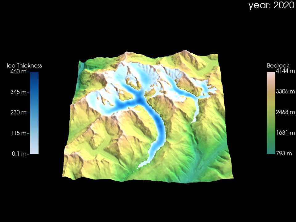
viz_zoomed = Glacier3DViz(
ds_glacier_zoomed, # the dataset for visualisation
camera_args={ # arguments for the point of view
'azimuth': -135, # rotate the map aroung the z-axis
'elevation': 20, # set the elevation above ground of the point of view
}
)
viz_zoomed.plot_year(2020)
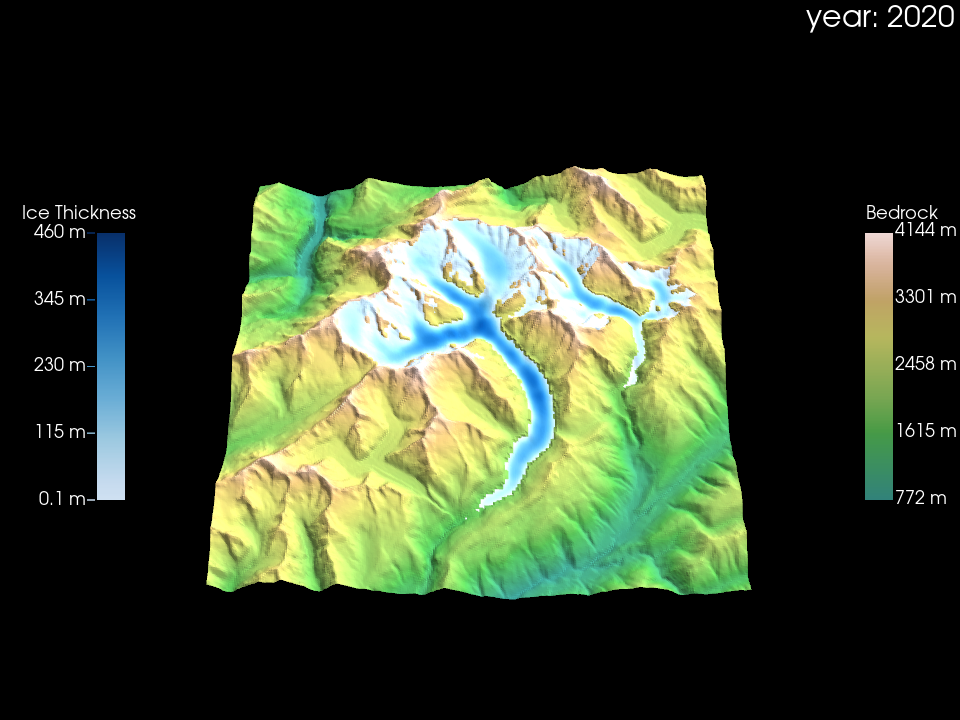
Or you can use the build in option for selecting a part of the center of your data. There are two options to do so presented in the following.
first option by giving the number of grid points
viz_zoomed_2 = Glacier3DViz(
ds_glacier, # the dataset for visualisation
x_crop=300, # how many grid points should be shown along the x-axis (centered)
# or a crop factor between 0 and 1, which crops in the percentage given by the crop factor.
y_crop=300, # how many grid points should be shown along the y-axis (centered)
# or a crop factor between 0 and 1, which crops in the percentage given by the crop factor.
camera_args={ # arguments for the point of view
'azimuth': -135, # rotate the map aroung the z-axis
'elevation': 20, # set the elevation above ground of the point of view
}
)
viz_zoomed_2.plot_year(2020)
second option by giving a crop factor:
viz_zoomed_3 = Glacier3DViz(
ds_glacier, # the dataset for visualisation
x_crop=0.65, # how many grid points should be shown along the x-axis (centered)
# or a crop factor between 0 and 1, which crops in the percentage given by the crop factor.
y_crop=0.5, # how many grid points should be shown along the y-axis (centered)
# or a crop factor between 0 and 1, which crops in the percentage given by the crop factor.
camera_args={ # arguments for the point of view
'azimuth': -135, # rotate the map aroung the z-axis
'elevation': 20, # set the elevation above ground of the point of view
}
)
viz_zoomed_3.plot_year(2020)
Change position and style of time label#
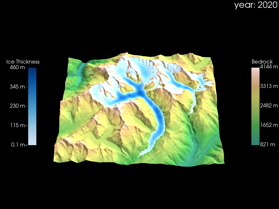
By default the shown year is displayed in the top right corner, but of course this also could be changed. See the PyVista documentation for all available options.
# look at the defaults
viz.text_time_args_default
{'text': 'year: {:.0f}',
'color': 'white',
'position': 'upper_right',
'viewport': True,
'font_size': 12,
'name': 'current_year'}
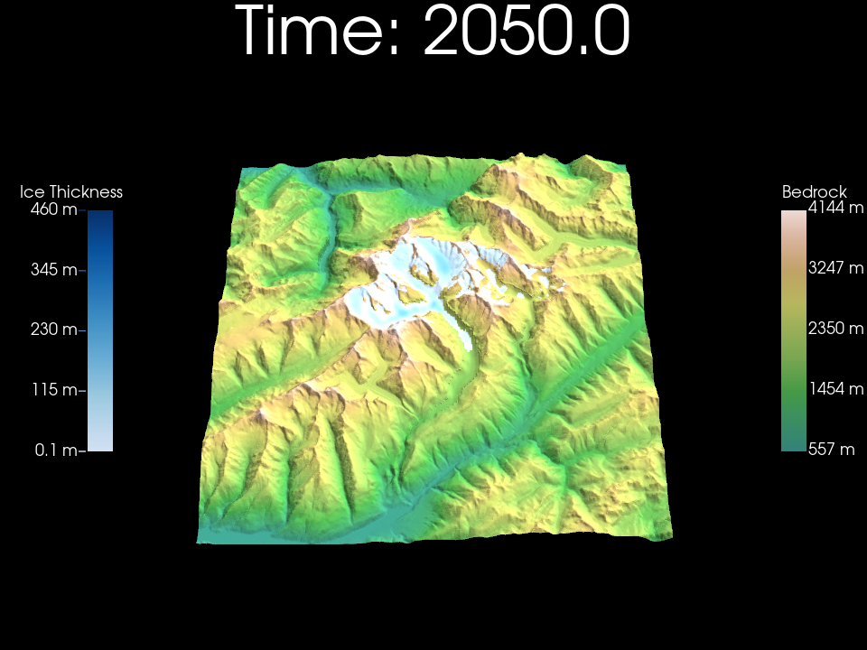
text_time_args_new = {
'text': 'Time: {:.1f}',
'position': 'upper_edge',
'font_size': 30,}
viz.plot_year(2050,
text_time_args=text_time_args_new)
What’s next?#
Check out Advanced Visualizations
Or back to the table of content