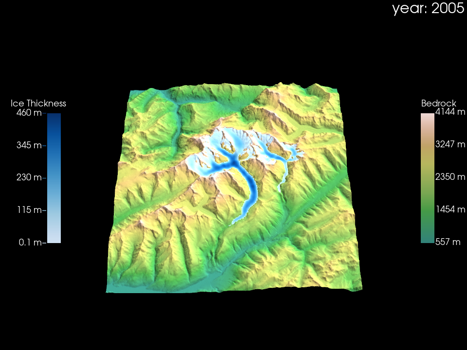
Advanced visualizations#
This tutorial showcases more advanced options available in Glacier:3D-Viz. It assumes that you have reviewed the previous tutorials and are somewhat familiar with the basic workflow.
Moving camera for animations#
An engaging effect can be achieved by changing your point of view during an animation. Currently, Glacier:3D-Viz supports two options for the camera trajectory, 'linear' or 'rotate'.
Linear camera movement#
With the option 'linear' you can define a start and an end point, with the camera moving in a straight line between them during the animation. Instructions on how to interactively determine the start and end points are provided in the general_styling tutorial. Here, we use this to define our start and end points:
viz.show() command currently does not display well in the Jupyter Book. You will get better results by executing the notebook locally. We are working on improving this!
import xarray as xr
from glacier3dviz.tools import Glacier3DViz
ds_glacier = xr.open_dataset("oggm_constant_climate_dummy_data.nc")
viz = Glacier3DViz(
ds_glacier,
camera_args={
'azimuth': -135,
'elevation': 20,
}
)
viz.show()
# change the point of view interactively above, and when your satisfied execute this cells for the coordinates
print(viz.get_camera_position())
[0.0, -3.0259101390838623, 48.929161071777344]
# copy the coordinates and define your start and end point
start_point = [-3.6, -6, 35]
end_point = [0.4, -1.2, 6.5]
# if you want to look at your current settings you can uncomment
#viz.plot_year(2020, camera_args={'position': start_point})
#viz.plot_year(2100, camera_args={'position': end_point})
# and finally create the animation
viz.export_animation(filename="dummy_moving_camera_animation.mp4",
camera_trajectory='linear',
kwargs_camera_trajectory={
'start_point': start_point,
'end_point': end_point
})

Rotating camera movement#
With the 'rotate' option, you can set up a rotating camera. You can define the 'start_angle' and 'end_angle' to control the rotation range of the camera. Additionally, you can adjust the 'camera_height' and 'camera_radius' (the distance from the center) to customize the camera’s position.
The camera will rotate around the map based on these parameters. To ensure the camera’s path forms a perfect circle (and not an ellipse), you can set a 'camera_radius_ref_axis' to either 'x' or 'y'. This scales all coordinates evenly along the chosen axis.
kwargs_rotate_camera_trajectory = dict(start_angle=180,
end_angle=300,
camera_height=10,
camera_radius=2,
camera_radius_ref_axis='x',
)
viz.export_animation(filename='dummy_rotating_camera_example.mp4',
camera_trajectory='rotate',
kwargs_camera_trajectory=kwargs_rotate_camera_trajectory
)

Side by side plots#
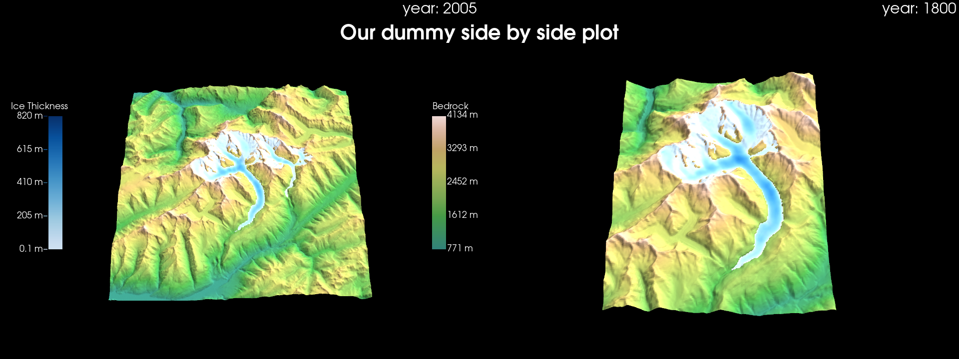
Displaying two simulations side by side can be useful, for example, to show the evolution of different scenarios or to compare two glacier models. To facilitate this, we implemented a small plotting function that allows you to add a single heading to the final side by side plot. The individual plots should be customized in the same way demonstrated in previous tutorials before merging them together. Let’s take a closer look:
import xarray as xr
from glacier3dviz.tools import Glacier3DViz, side_by_side_visualization
ds_oggm = xr.open_dataset("oggm_constant_climate_dummy_data.nc")
viz_oggm = Glacier3DViz(
ds_oggm,
camera_args={
'azimuth': -135,
'elevation': 20,
}
)
ds_igm = xr.open_dataset("igm_dummy_data.nc")
viz_igm = Glacier3DViz(
ds_igm,
x='x',
y='y',
time='time',
topo_bedrock='topg',
ice_thickness='thk',
time_var_display='time',
camera_args={
'azimuth': -135,
'elevation': 20,
}
)
side_by_side_visualization(
[viz_oggm, viz_igm], # a list of Glacier3DViz objects to show
shape=(1, 2), # how they should the layout look like (also more than two is possible)
title='Our dummy side by side plot', # the title text
kwargs_title={'fontsize': 40, # some arguments to customize the title
'color': (1, 1, 1),
'position': (0.5, 0.93),
},
filename_plot=f'dummy_side_by_side_plot.png', # if you want to save a plot, provide a path here
plot_year=2000, # the year which should be plotted, is taken from first object in the list
filename_animation=None, # if you want to save an animation, provide a path here
framerate=80, # framerate of the animation
quality=10, # quality of the animatoin
# moving_camera_start_and_end_point=moving_camera_start_and_end_point, # see moving camera section above
)

This plot contains only one colorbar for each element. You need to adjust the individual elements to create a cohesive overall appearance for a side-by-side plot. Instructions on how to customize individual plots are provided in the previous tutorials.
Add images as insets#
After creating an animation, you may want to include additional information, such as a map showing the glacier’s location or the logo of your university or company. For example, in this section, we add a globe to highlight the location of our glacier:
import xarray as xr
from glacier3dviz.tools import Glacier3DViz, plot_centered_globe, add_inset_with_ffmpeg
ds_glacier = xr.open_dataset("oggm_constant_climate_dummy_data.nc")
plot_centered_globe(ds_glacier,
filename='dummy_globe.png')

And now, we can incorporate this into our videos using FFmpeg. You have the option to scale the image (scale_factor) and set its position (position).
For position, you define the top-left corner of the image as 'x:y'. You can use W/H (width/height of the video) and w/h (width/height of the image) to calculate the desired placement. Example positions include:
Top-left:
'0:0'Centered:
'(W-w)/2:(H-h)/2'Bottom-right:
'W-w:H-h'
add_inset_with_ffmpeg(
main_video=f'dummy_animation.mp4',
inset_image=f'dummy_globe.png',
output_video=f'dummy_animation_with_map.mp4',
position='20:20', # top-left, with 20 pixels space to the edges
scale_factor=1, # here you can resize the image
)
Overlay added successfully! Output saved to 'dummy_animation_with_map.mp4'.
What’s next?#
Check out General styling of 3D visualisations
Or back to the table of content